
TL;DR
- 100K sensors, one value roughly every ~740ms, 11 hours → ~6B rows, ingested continuously via Zerobus using Protobuf messages (triples of sensor_name, event_timestamp, value). Total ingestion cost, billed as Lakeflow Connect usage: ~$20.
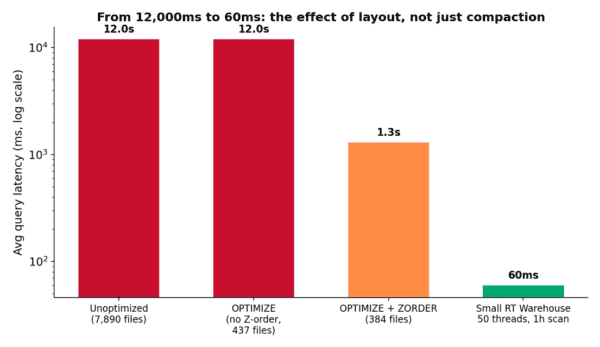
- Left unoptimized, this produced 7,890 tiny files — one every 5 seconds as described in the Zerobus documentation — and single-sensor queries averaged 12 seconds.
- Running OPTIMIZE alone (no Z-order) compacted the table to 437 files but query time didn’t improve at all indicating the issue has to do with the actual data layout within the files.
- Adding Z-ORDER on sensor_name, event_timestamp dropped latency from 12s to roughly 1s — instantly, mid-benchmark, while the OPTIMIZE job was still running.
- Post Z-order, 20 concurrent threads sustained 1.3s average latency at 14.8 queries/sec, querying full sensor history.
- On a Small RT Warehouse, running a much smaller one-hour range scan instead of full history, we pushed ~735 q/s at 50 threads, with average end-to-end latency of just ~60ms. That’s roughly a 20x latency improvement over the full-history query, but a big part of that comes from asking for 11x less data per query (see below), not from the warehouse alone.
What is Zerobus?
Zerobus Ingest This link opens in a new tab is Databricks’ push-based streaming ingestion API, part of Lakeflow Connect. It writes data directly into Unity Catalog Delta tables at high scale — no Kafka cluster to run, no partitions or brokers to manage. A producer opens a gRPC (or REST) stream, sends schema-compatible messages (JSON, Protobuf, or Arrow), and Zerobus makes each record durable and lands it in the target Delta table, typically within 5 seconds. Scaling is just a matter of opening more connections; there’s no capacity planning on the ingestion side. If you want to go deeper, the Zerobus concepts page This link opens in a new tab covers streams, servers, and supported message types, and the SDK repository This link opens in a new tab has client examples in Python, Rust, Java, Go, and TypeScript.
The setup
We used Zerobus to simulate a fleet of 100,000 IoT sensors, each emitting a single value roughly every ~660 milliseconds, resulting to almost 6 billion records. Each message was sent as a compact Protobuf record — just sensor_name, event_timestamp, and value — and the whole 11-hour ingestion run was billed at roughly $20 under the Lakeflow Connect SKU. With a price per GB of 0.062 Euro this means a total of 323GB of data ingested, roughly 58 bytes per record which makes sense in uncompressed form. I used sensor names in the form ‘sensor_<id>’ which actually costs me 2.40 Euro compared to simply sending the <ID>. So my lesson learned, minimize what you are sending as these things do add up in the long run… (duh).
During the ingestion we queried the Delta table for recent data for a random sensor name (0 to 99.999) like:
SELECT * FROM sensor_readings <br>WHERE sensor_name = ‘sensor_X’ AND event_timestamp > now() - INTERVAL 10 MINUTESThe data we could query lagged by ~5 seconds which makes sense given the way Zerobus writes data.
Act 1: The Small File Problem
Zerobus, by design, commits frequently to keep end-to-end latency low. In our run that meant one file roughly every 5 seconds, and over 11 hours that adds up fast: 7,890 files, each holding a random, unsorted slice of whichever sensors happened to report in that window.
On a Small RT Warehouse, “give me the last 10 minutes for a sensor” queries executed with roughly 3–5 second round trip. Not extremely fast but these queries always required the warehouse to fetch the latest files from cloud storage. But anything that had to reach further back kept getting slower as the file count grew, and a full table scan for a single sensor was where things fell apart. We benchmarked this with 2 concurrent threads, each pulling a single sensor’s complete ~60,000-record history: average query time: 12 seconds.
With ~6B rows scattered across 7,890 files with no optimization, every sensor’s data was spread across effectively all of them — the query engine had no choice but to open nearly every file to reconstruct one sensor’s timeline.
Act 2: OPTIMIZE Alone Isn't Enough
The obvious first move is to run OPTIMIZE and compact those thousands of small files into fewer, larger ones. We did — no partitioning, no Z-order, just plain file compaction from 7,890 to 437 files.
We re-ran the identical 2-thread, single-sensor, full-history benchmark expecting some improvements but average query time remained 12 seconds.
Fewer files didn’t help because the problem was not only the number of files but also the file composition (i.e. parquet row group layout). Each of the 437 compacted files still contained a random shuffle of all 100,000 sensors, so answering “give me sensor X’s history” still meant scanning every single file. Our working theory is that even with far fewer files, the query engine still had to open and filter and decompressing thousands of Parquet row groups internally, each one still holding a random mix of sensor values — so the same amount of irrelevant data had to be read and discarded, just with less file-open overhead than before.
Act 3: Z-ORDER, and the Moment Everything Changed
Next we ran:
OPTIMIZE sensor_readings ZORDER BY (sensor_name, event_timestamp)on serverless compute. It took about 2 minutes and brought the file count down slightly further, from 437 to 384 files — a much smaller change in file count than the OPTIMIZE step, but a completely different change in data layout: rows are now physically co-located by sensor, then by time.
We had the benchmark running continuously through this operation, and the result is the best chart from this whole experiment:
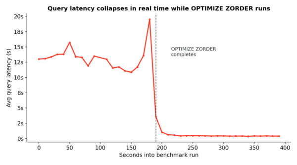
For roughly the first three minutes, average query latency by a single thread was trending down towards the 11s seen before as the old file layout is still what’s being read. Then, the query time increases a bit, assumingly to get the newly created files, after which the query execution time decreases down to ~400–500ms by a single thread.
Once the dust settled, we ran a clean benchmark against the fully Z-ordered table with 20 concurrent threads, still pulling each sensor’s full history:
- Average latency: 1.3 seconds
- Throughput: 14.8 queries/second
Putting the whole journey on one chart, on a log scale, makes the shape of the story clear:
Act 4: How Far Can the RT Warehouse Go?
With the table properly laid out, we shifted the question from “is this fast enough for one query” to “how much concurrent queries can a Small RT Warehouse actually execute.” We switched the query to only get one hour of data for a random sensor (~5,500 records per sensor, about 11x less data than a full-history pull) and ramped up concurrent threads.
At 50 threads, we sustained:
- ~735 queries/second
- Average latency ~60ms, within a few milliseconds of the platform’s reported minimum response time of ~50ms
- Zero failed requests over the full run
Pushing past 50 threads started returning ‘429 — Too Many Requests, resource is exhausted errors’, which is the warehouse telling us we’d found its ceiling for this size tier rather than a query-plan problem.
Takeaways
With the table properly laid out, we shifted the question from “is this fast enough for one query” to “how much concurrent queries can a Small RT Warehouse actually execute.” We switched the query to only get one hour of data for a random sensor (~5,500 records per sensor, about 11x less data than a full-history pull) and ramped up concurrent threads.
- Zerobus makes high-frequency, near-real-time ingestion easy and cheap — but will produce many small files by design. Our full 11-hour, ~6B-row run cost about $20 in Lakeflow Connect charges. Minimize what you are sending to lower your bill
- File count is not the same problem as data layout. OPTIMIZE without Z-order fixed the former and left query time completely unchanged, because the latter — random sensor distribution across files (and, we believe, across Parquet row groups) — was the actual bottleneck.
- OPTIMIZE ZORDER on the right columns turned a full-history scan from 12 seconds into ~1.3 seconds, and the transition happens the instant the job finishes, not gradually. Probably better to use Liquid Clustering but I did not have the time to run a lot of queries, wait a bit and then optimize to do it again (I expect liquid clustering to get to the same performance for this specific set of queries).
- A properly laid-out table plus a Small RT Warehouse can comfortably serve hundreds of queries per second at tens-of-milliseconds latency for right-sized queries (here, one-hour scans) — good enough to sit under a live dashboard or an alerting pipeline directly on top of streaming data, without a separate serving layer.
In 2022 I benchmarked Databricks SQL in the context of an IoT monitoring solution. Back then it was discarded as it could not keep up, and instead we landed on Azure Data Explorer. This matched the use case perfectly but isn’t a generic data platform solution. Looking at my numbers from four years ago it seems ADX still performs better than RT and at a lower price point when purely looking at compute costs. But having a truly unified solution is also worth a lot. I don’t know if that decision for ADX would have been so clear-cut if Zerobus and RT Warehouses had existed back then.